Mass Audio (tm) - Machine Learning
Mass Audio (tm) is a module in the school of Techbotism Audio production
This is a work in progress as I figure out Machine Learning from scratch. I literally need to google at least one word per sentence in everything I read.
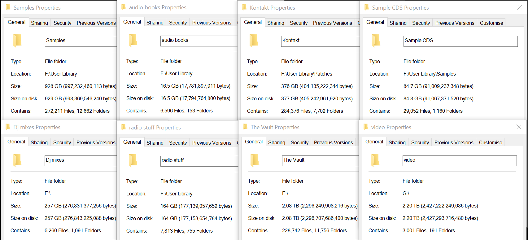
Over the years we've collected over 8,000 albums. Since we joined Bandcamp 18 months ago we've amassed another 10,000 albums.
928 gigabytes of samples,
376 gigabytes of multisamples,
84 gigabytes of Sampl CDs,
257 gigabytes of djs mixes ,
164 gigabytes of Radio Stuff
I want a machine Learning AI thing to analize all this audio break it down into units that are categorisable. Then when I choose a piece of audio, it recreates new pieces of audio isungmy chosen one as a staring point and replacing each of the untis within the audio with a similar unit based on whatever options are availble. This is then broadcast as the sum of all audio eminating from the planet and bounced back via the hijacked EMC23 pirate satellite
http://www.justinsalamon.com/uploads/4/3/9/4/4394963/cramer_looklistenlearnmore_icassp_2019.pdf
So what are we talking here? Well Audio Word Embeddings (AWE) are patterns for words spoken at variable speed, so we're talking dynamic time warpng. (two people start walking beside each other at slightly different speeds- the defining pattern remains the same). So with L3 we are talking Deep Audio Embeddings or patters for sounds. So while AWE might be good for voice recogition DAE might be good for sound recognition, pitch recognition and maybe instrument separation in a mix I dunno. this is my first day at school.
What I woud hope to do is break my Mass Audio (tm) collection into DA Embeddings and from them analyse and auto generate ambient, experiment and avant garde music. I would hope to go deep into convolution techniques
https://github.com/marl/openl3
Step 1: Install Python 3.7 ( 3.9 prevents h5py-3.2.1.dll )
Step 2: Install tensor flow 1.14 (not tensorflow 2)
pip install "tensorflow<1.14"
Step 3: Pip install openl3
pip install openl3
Open L3 Tutorial:
https://openl3.readthedocs.io/en/latest/tutorial.html
Using the Command Line Interface (CLI)
Extracting audio embeddings
To compute embeddings for a single audio file via the command line run:
$ openl3 audio /path/to/file.wav
This will create an output file at /path/to/file.npz.
You can change the output directory as follows:
$ openl3 audio /path/to/file.wav --output /different/dir
This will create an output file at /different/dir/file.npz.
You can also provide multiple input files:
$ openl3 audio /path/to/file1.wav /path/to/file2.wav /path/to/file3.wav
which will create the output files /different/dir/file1.npz, /different/dir/file2.npz, and different/dir/file3.npz.
You can also provide one (or more) directories to process:
$ openl3 audio /path/to/audio/dir
https://github.com/marl/urbanorchestra
UrbanOrchestra
Making music from urban environments!
Install miniconda
- Visit page at:
https://conda.io/miniconda.html
Download MedleyDB dataset
- Download request form is at:
http://medleydb.weebly.com/download-form.html
Download Urban-SED dataset
- Download request form is at:
http://urbansed.weebly.com/download.html
Download VGGish models:
cd ./audiosetcurl -O https://storage.googleapis.com/audioset/vggish_model.ckptcurl -O https://storage.googleapis.com/audioset/vggish_pca_params.npzcd ..
Setup and activate conda environment
conda env create -f urbanorchestra.ymlsource activate urbanorchestra
Define path to datasets in Conda environment
export URBAN_SED_PATH = "/path/to/local/MedleyDB"export MEDLEYDB_PATH = "/path/to/local/MedleyDB"
Install MedleyDB package
git clone https://github.com/marl/medleydb.gitcd medleydbpython setup.pycd ..
Tensorflow:
Machine Learning:
- Feature: The input(s) to our model
- Examples: An input/output pair used for training
- Labels: The output of the model
- Layer: A collection of nodes connected together within a neural network.
- Model: The representation of your neural network
- Dense and Fully Connected (FC): Each node in one layer is connected to each node in the previous layer.
- Weights and biases: The internal variables of model
- Loss: The discrepancy between the desired output and the actual output
- MSE: Mean squared error, a type of loss function that counts a small number of large discrepancies as worse than a large number of small ones.
- Gradient Descent: An algorithm that changes the internal variables a bit at a time to gradually reduce the loss function.
- Optimizer: A specific implementation of the gradient descent algorithm. (There are many algorithms for this. In this course we will only use the “Adam” Optimizer, which stands for ADAptive with Momentum. It is considered the best-practice optimizer.)
- Learning rate: The “step size” for loss improvement during gradient descent.
- Batch: The set of examples used during training of the neural network
- Epoch: A full pass over the entire training dataset
- Forward pass: The computation of output values from input
- Backward pass (backpropagation): The calculation of internal variable adjustments according to the optimizer algorithm, starting from the output layer and working back through each layer to the input.
https://github.com/mtobeiyf/audio-classification
https://github.com/karolpiczak/ESC-50
https://opensource.com/article/19/9/audio-processing-machine-learning-python
https://medium.com/comet-ml/applyingmachinelearningtoaudioanalysis-utm-source-kdnuggets11-19-e160b069e88
https://github.com/meyda/meyda
https://github.com/tyiannak/pyAudioAnalysis
https://medium.com/@ageitgey/machine-learning-is-fun-part-6-how-to-do-speech-recognition-with-deep-learning-28293c162f7a
https://towardsdatascience.com/urban-sound-classification-part-1-99137c6335f9
https://www.analyticsvidhya.com/blog/2017/08/audio-voice-processing-deep-learning/
http://www.practicalcryptography.com/miscellaneous/machine-learning/guide-mel-frequency-cepstral-coefficients-mfccs/
https://github.com/jameslyons/python_speech_features
https://hackernoon.com/audio-handling-basics-how-to-process-audio-files-using-python-cli-jo283u3y
UltrasoundAudio8k
Sound Classification using Librosa, ffmpeg, CNN, Keras, XGBoost, Random Forest.
Dataset and its structure
NOTE: multiple_model_mfcc.ipynb is best model
- We can use Urban Sound Classification dataset which is quite popular.
- Whichever dataset you are using, it is important to understand its structure and how to extract required features out of them.
- For UrbanSound8K dataset, it can be downloaded using the following link. It downloads a compressed tar file of size around 6GB.
- On extracting it, it contains two folders named 'audio' and 'metadata'.
- Audio folder contains 10 folders with name fold1, fold2 and so on, each having approximately 800 audio files of 4s each.
- Metadata folder contains a .csv file having various columns such as file_id, label, class_id corresponding to label, salience etc.
- Complete description can be found here
Research Paper and Resources to follow
- https://github.com/meyda/meyda/wiki/audio-features
- https://github.com/tyiannak/pyAudioAnalysis/wiki/3.-Feature-Extraction
- https://medium.com/@ageitgey/machine-learning-is-fun-part-6-how-to-do-speech-recognition-with-deep-learning-28293c162f7a
- https://towardsdatascience.com/urban-sound-classification-part-1-99137c6335f9
- https://www.analyticsvidhya.com/blog/2017/08/audio-voice-processing-deep-learning/
Library To Use
We can use librosa library which can be installed using
pip install librosa
It uses ffmpeg as backend to convert and read some of the audio files. So to install ffmpeg, you can use
apt-get install ffmeg
Librosa library can read audio files and convert them to there amplitude values for each sample of audio. Let us say there is an audio file of 4s and sampling rate of audio file is 22050 Hz. This means that audio file is made using amplitude samples such that 22050 samples of amplitudes are recorded in each second. Hence a 4s audio file with sampling rate 22050 can be expressed as an array of 4*22050=88200 size
How to Load Audio Files and Extract Features
Using load method of librosa library, we can read audio files. It takes file path as input and returns an array having amplitude samples along with sampling rate of file.
Librosa library has many methods already build to extract features mentioned in resources which then returns another array of features. We can use various combinations of those features. This is something you can play around and try how and which features like mfcc, spectral features, energy etc affect the classification of audio.
For eg, in first stage you can extract only mfcc features and then build up a model and check the accuracy. Then try the same with other features. In order to further improve accuracy, you can also try to use more than one type of features and check the results.
Using CNN to classify sound
This is a very classical way of sound classification as it is observed that similar type of sounds have similar spectrogram (read resource 3 to understand more about spectrogram). A spectrogram is a visual representation of the spectrum of frequencies of sound or other signal as they vary with time. And thus we can train a CNN network which takes these spectrogram images as input and using it tries to generalize patterns and hence classify them.
MFCC Guide
The first step in any automatic speech recognition system is to extract features i.e. identify the components of the audio signal that are good for identifying the linguistic content and discarding all the other stuff which carries information like background noise, emotion etc.
The main point to understand about speech is that the sounds generated by a human are filtered by the shape of the vocal tract including tongue, teeth etc. This shape determines what sound comes out. If we can determine the shape accurately, this should give us an accurate representation of the phoneme being produced. The shape of the vocal tract manifests itself in the envelope of the short time power spectrum, and the job of MFCCs is to accurately represent this envelope. This page will provide a short tutorial on MFCCs.
Mel Frequency Cepstral Coefficents (MFCCs) are a feature widely used in automatic speech and speaker recognition. They were introduced by Davis and Mermelstein in the 1980's, and have been state-of-the-art ever since. Prior to the introduction of MFCCs, Linear Prediction Coefficients (LPCs) and Linear Prediction Cepstral Coefficients (LPCCs) (click here for a tutorial on cepstrum and LPCCs) and were the main feature type for automatic speech recognition (ASR), especially with HMM classifiers. This page will go over the main aspects of MFCCs, why they make a good feature for ASR, and how to implement them.
www.practicalcryptography.com/miscellaneous/machine-learning/guide-mel-frequency-cepstral-coefficients-mfccs/